


SPC control limits are the two lines on a control chart, the upper (UCL) and the lower (LCL), that show how much your process varies when only normal, random causes are at work. You calculate them from your own process data, usually as the centre line plus and minus three standard deviations. A point outside them is a signal to investigate, not a verdict that a part is bad.
This guide is for production managers, quality engineers and plant automation teams who already draw control charts, or want to start, and need the limits to mean something. We cover how the limits are set, how much data you need, the most common mistake (mixing them up with specification limits), and when to recalculate them.
A control chart plots a measurement over time: a diameter, a fill weight, a torque value, a cycle time. Three lines sit on the chart: the centre line (the process average) and the upper and lower control limits. The idea behind statistical process control is to compare what the process is doing today with what it did before, so that you notice a change early.
The limits are the boundary of expected variation. If points scatter randomly between them, the process is behaving as it usually does. If a point falls outside, or the points form an unusual pattern, something has probably changed: a worn tool, a new material batch, a different operator setup.
That is all the limits say. They do not say whether a part meets the drawing. That is the job of specification limits, and the difference matters enough to have its own section below.
The standard placement is three standard deviations above and below the centre line. According to ISO 7870-2:2023, this captures about 99.73% of the data from a stable process. The chance of a false alarm from random variation alone is therefore about 0.27%, roughly 3 points in 1,000.
In practice that is a good balance. Set the limits tighter and operators chase noise. Set them wider and real shifts hide inside the band.
3σ is a default, not a law. The same standard says management should choose the k-sigma value by weighing the cost of investigating a signal against the consequence of missing a shift. If missing a defect is very expensive, for example in a safety-relevant characteristic, you can use narrower limits and accept more false alarms. If every stoppage costs a lot and defects are cheap to catch downstream, you may stay with 3σ.
Write the decision down, with the reasoning. When an auditor or a new quality engineer asks why the limits sit where they do, the answer should not be “that is what the software did”.
The formula depends on the data. An individuals chart (one reading per sample) estimates variation from the moving range. An X-bar and R chart estimates it from the range within each subgroup. Attribute charts (p, np, c, u) use binomial or Poisson models. The 3σ logic is the same in each case. If you are choosing which chart fits which measurement, our guide on SPC in production and the charts your team can use this week walks through the options.
SPC has two phases, as described in ASTM E2587. In Phase I you use historical data to calculate the initial limits and check whether the process is stable. In Phase II you use those limits for real-time monitoring. You should move to Phase II only once Phase I confirms a state of statistical control.
This order is where many plants go wrong. They calculate limits from the first few samples, switch on alarms and then wonder why operators ignore them.
The NIST/SEMATECH handbook follows Shewhart’s rule of thumb: at least 25 subgroups, typically of size 4, before you conclude that a state of control has been reached. For charts with one observation per subgroup, aim for at least 30 points. With fewer, the estimate of variation is poor and false alarms are likely.
A simple Phase I routine:
The quality of this step depends on trustworthy historical data. A guide on the role of control in industrial processes (in Italian) explains from the shop floor angle why data gathered consistently over time is what makes later monitoring meaningful. Manual transcription is the weak link here: a mistyped value can create a false outlier or hide a real one.
This is the most common confusion in SPC, and it leads to bad decisions in both directions.
| Control limits | Specification limits | |
|---|---|---|
| Source | Your process data | Drawing, standard or customer |
| Question answered | Is the process stable? | Is the part acceptable? |
| Changes when | The process changes | The requirement changes |
| Applies to | Subgroup averages or individual points on a chart | Individual parts |
The NIST handbook on process capability compares the output of an in-control process with the specification limits using capability indices. The order matters: first stability, then capability. If a process is in statistical control but still produces parts outside specification, it is simply incapable. More charting will not fix that. The process design has to change, for example the tooling, the material or the setting window.
The reverse also happens. A process can sit comfortably inside the specification while drifting. The control limits are what show the drift before parts fail.
Subgroup averages vary less than individual parts. If you draw the specification on a chart of averages, you will believe the process is safer than it is. Keep specification limits for histograms and capability analysis, and keep control limits for the chart.
Once the process is stable, compare its spread with the specification using Cp and Cpk. Waterloo’s overview of capability indices notes that in the automotive sector a Cpk of 1.33 is a common minimum benchmark, with higher targets such as 1.67 often applied to significant characteristics. Below 1.33, corrective action such as extra inspection or process changes is generally expected. Check your own customer’s requirement, since it can differ by customer and characteristic.
A point beyond a limit is the clearest signal, but not the only one. Common additional rules look for:
Each extra rule increases sensitivity and also the false alarm rate, so use a small, agreed set. Most plants do well with the out-of-limit rule plus one or two run rules, and add more only for critical characteristics.
ASTM E2587 stresses the value of an Out-of-Control Action Plan (OCAP): a defined procedure for what the production team does when a point falls outside the limits. Without it, monitoring becomes firefighting. The chart gives a signal, but the value comes from the structured investigation that follows.
A workable OCAP fits on one page per chart:
Our article on enforceable quality control checkpoints on the shop floor shows how to tie such actions to a specific station so they actually happen.
Resist the urge to refresh limits automatically each week. The NIST guidance suggests revising limits only for a good reason. Two are valid: you have gathered enough new data (at least about 30 new points) to estimate variability better, or a major and permanent process change has occurred, such as an equipment overhaul or a different raw material. Constant recalculation lets the limits follow the drift, so the chart can no longer detect a shift from the baseline.
A short decision rule:
| Situation | Recalculate? |
|---|---|
| One point outside the limits, cause found and fixed | Ne |
| Process improvement that reduced variation permanently | Yes, after enough new data |
| Machine rebuilt or new supplier material | Yes, start a new Phase I |
| Operators find the limits “too tight” | No. Check the process and the measurement first |
| New data confirms the same variation | Ne |
Keep a log: date, reason, old and new limits, who approved. It makes audits easier and prevents silent changes.
We build manufacturing execution software, so we see the same pattern in many factories: the statistics are rarely the problem. The problem is the data path. Values are written on paper, typed into a spreadsheet at the end of the shift and charted the next morning. By then the signal is hours old, and the 25 subgroups needed for Phase I take months to collect and are full of transcription errors.
When measurements come straight from the equipment and are timestamped by machine, shift and product, three things change. Phase I can be done in days from clean data. Stratifying by machine or lot becomes a filter rather than a project. And a signal reaches the right person while the cause is still on the line.
Our advice is to start with one critical characteristic, set the limits properly, write the OCAP and prove that the team reacts. Then extend. A few charts that people act on are worth more than a hundred that nobody reads.
— Andraž
If you want live control charts fed directly from your machines, with KPIs, downtime and quality parameters in one view, Mestric™ MES connects to production equipment and collects data automatically. We show how this works on connected machinery in a demonstration. For the wider context of how real-time quality data supports your decisions, see our overview of production quality monitoring.
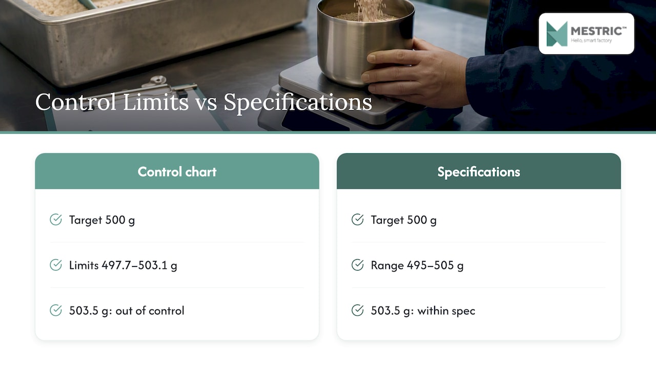
Imagine a filling line where the target is 500 g and the tolerance is 495 to 505 g. You collect 25 subgroups of 4 bottles, taken every 30 minutes across two shifts. The grand average is 500.4 g and the average within-subgroup variation gives a standard deviation of the subgroup mean of about 0.9 g. Your 3σ limits on the X-bar chart are then about 497.7 and 503.1 g.
These figures are illustrative, not from a real plant. Notice what they show. The control limits (497.7 to 503.1 g) are narrower than the tolerance (495 to 505 g) because they apply to averages of four. A subgroup average at 503.5 g is out of control while still well inside the specification. That is the early warning you want: investigate now, while no part is scrap.
Now suppose the process were shifted so that the average sat at 504 g. The chart would signal at once, and the capability analysis would tell you that even a stable process at this setting would produce out-of-specification bottles. Two different problems, two different tools.
Control limits are calculated from your process data and show what the process normally does. Specification limits come from the drawing or the customer and define an acceptable part. A stable process can still produce parts outside specification, and a process inside specification can still be drifting.
Because it balances false alarms and missed shifts. For a stable process, 3σ limits give roughly a 0.27% chance of a false alarm per point, according to ISO 7870-2:2023. You can use a different k-sigma if the cost of missing a defect justifies more false alarms.
Use at least 25 subgroups, typically of size 4, or around 30 points for an individuals chart. Fewer samples give unreliable limits and more false alarms. Check the process is stable before using the limits for live monitoring.
Only when there is a reason: a permanent process change such as new equipment or material, or enough new data (about 30 points or more) to improve the estimate. Do not recalculate after every out-of-limit point, because that hides the shifts the chart exists to detect.


 069 763 552