The single most effective first move is to adopt an SLO-driven monitoring approach that prioritises p95/p99 latency, real user telemetry, and error-budget burn-rate alerts. Before you instrument anything, define what “working” means for your users, then build your telemetry around that definition.

Three immediate next steps:

1. Identify a small number of critical user journeys (for example, checkout, login, or a key API path) and write SLOs for each.
2. Instrument those paths to emit histogram metrics and distributed traces.
3. Set an initial burn-rate alert and wire it to a dashboard your on-call team can read in under 30 seconds.

Quick-start checklist:

• Agree on UTC as the timestamp standard across all services.
• Enable structured logging on at least one critical service.
• Create one SLO dashboard with error-budget burn rate visible.
• Add a deploy marker to your dashboard so you can correlate releases with performance shifts.
• Document a one-page runbook for your first alert.

Table of Contents

• What is real-time performance monitoring?
• How a real-time monitoring pipeline works
• What business outcomes does real-time monitoring deliver?
• Which metrics should you monitor?
• Telemetry architecture and SLO-driven design for UK organisations
• How do you instrument, build dashboards, and configure alerts?
• Recovery testing, alert tuning, and operational readiness
• Implementation checklist: timeline, roles, and cost drivers
• Which tooling categories do you need?
• Your 90-day starter plan
• Key takeaways
• The case for SLO-first monitoring: a practitioner perspective
• Mestric brings real-time monitoring to your factory floor
• Useful sources for further reading

What is real-time performance monitoring?

Real-time performance monitoring is the continuous collection, low-latency processing, and action on telemetry as events occur, rather than waiting for a batch report to land the next morning. The distinction matters: periodic reporting tells you what happened; real-time monitoring tells you what is happening now, so you can act before users notice a problem.

The scope covers five telemetry types:

• Metrics — numeric time-series data (CPU, request rate, error count); best for alerting and trending.
• Logs — structured or semi-structured event records; best for root-cause investigation.
• Traces — distributed request spans across services; best for latency diagnosis and dependency mapping.
• Real user monitoring (RUM) — browser and mobile telemetry from actual users; best for front-end experience and segmentation.
• Synthetic checks — scripted probes from fixed locations; best for baseline availability and regression detection.

Business KPIs tied to user journeys (conversion rate, order throughput, session abandonment) belong in scope too. Monitoring only infrastructure components without linking them to user outcomes is a common gap that leaves decision-makers without the context they need.

Real-time vs near-real-time vs historical analysis

The hot/warm/cold architecture is the standard pattern for balancing query speed against storage cost. Hot analysis must support fast indexing and querying; warm is for correlation; cold is for long-term trend analysis and forecasting.

How a real-time monitoring pipeline works

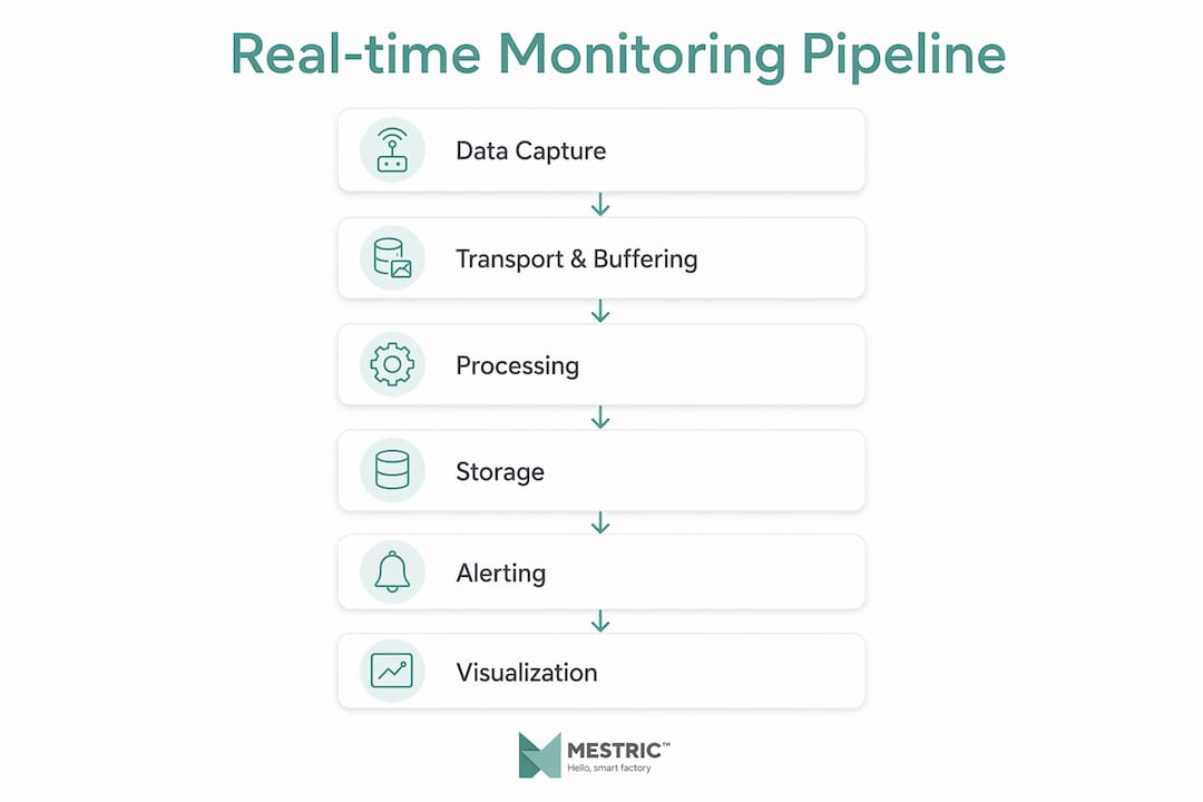
Every monitoring system follows the same logical flow: instrument your code and services, collect the telemetry, ship it through a resilient pipeline, process it in a hot tier, route older data to long-term storage, and surface everything via dashboards, alerts, and traces.

Instrumentation primitives

• Histograms — record the distribution of values (latency, payload size) so you can compute p50, p95, and p99 at query time.
• Counters — monotonically increasing values for request counts, error counts, and throughput.
• Structured logs — JSON-formatted event records with consistent field names (service, trace_id, level, message) for reliable querying.
• Spans — start/end timestamps with metadata that represent a unit of work within a distributed trace.

Transport and buffering

Telemetry pipelines fail under load if you do not design for backpressure. Use a message queue (Kafka, RabbitMQ, or a cloud-native equivalent) between your collectors and your processing layer. Configure retries with exponential back-off and set explicit queue depth limits so a downstream outage does not cascade into data loss.

Processing and storage

Aggregate histograms server-side before writing to your time-series database (TSDB) so you can compute global percentiles across multiple instances. Apply head-based or tail-based sampling to traces: head-based sampling is simpler but misses rare errors; tail-based sampling retains interesting traces (errors, slow outliers) at the cost of more processing. For most UK production systems, a sampling rate of 1–10% for normal traffic with 100% retention for errors is a practical starting point.

Pro Tip: Always store all telemetry timestamps in UTC. Mixed timezone offsets in a distributed system make event correlation unreliable and can cause alert conditions to appear hours after the actual incident.

The pipeline in summary:

1. Services emit metrics (histograms, counters), structured logs, and spans.
2. A collector agent (running on the host or as a sidecar) batches and forwards telemetry.
3. A message queue buffers the stream and absorbs traffic spikes.
4. A processing layer aggregates metrics, indexes logs, and samples traces.
5. Hot-tier storage (fast TSDB, indexed log store) serves dashboards and alerts.
6. A cold-tier store (object storage) receives compacted data for long-term analysis.

Percentile-based latency tracking using histograms is the only reliable way to surface these outliers at scale.

What business outcomes does real-time monitoring deliver?

The business case for real-time monitoring rests on four measurable outcomes: reduced mean time to recovery (MTTR), preserved revenue during incidents, improved customer retention, and fewer production incidents overall.

When your on-call engineer receives a burn-rate alert with a pre-linked runbook, diagnosis starts in seconds rather than minutes. Faster diagnosis directly compresses MTTR. For e-commerce and SaaS businesses, every minute of degraded checkout performance translates into lost conversions, so the financial case is direct.

Stakeholder benefits by role:

• Engineering teams — fewer pages at 2 AM, faster root-cause analysis, and clear SLO targets to design against.
• Site reliability and operations — error-budget visibility that supports data-driven release decisions.
• Product management — user journey telemetry that connects technical health to feature adoption and conversion.
• Executive leadership — uptime and SLO compliance reports that translate technical reliability into business risk language.

Real-time production monitoring in manufacturing contexts adds a further dimension: connecting machine-level telemetry to production KPIs means downtime events surface on a dashboard before they become a shift-level problem. The seven proven benefits of real-time monitoring in manufacturing include reduced stoppages, improved quality yield, and lower cost per unit, all of which follow directly from faster detection and response.

SLOs as the primary driver for alerting and monitoring strategy is the principle that underpins this outcome-first approach.

Which metrics should you monitor?

The four golden signals, first described in Google’s Site Reliability Engineering practice, give you a complete picture of any service’s health.

Beyond the golden signals, include business KPIs: order completion rate, session duration, and payment success rate. These translate SLO breaches into language that resonates with non-technical stakeholders.

Why p99 matters more than average

Averages (p50) hide poor experiences. If your average response time is 300 ms but your p99 is 4 seconds, one in every hundred requests is severely degraded. At scale, that is thousands of users per hour. Use histograms to aggregate and compute global percentiles across instances; a simple average across instance averages is mathematically incorrect and will understate tail latency.

SLO templates

# Availability SLO
service: payment-api
objective: 99.9% of requests succeed (non-5xx) over a 30-day rolling window
error_budget: 0.1% = ~43 minutes/month

# Latency SLO
service: checkout-page
objective: p99 response time < 2 s for 99.5% of requests over a 30-day window
error_budget: 0.5% of requests may exceed 2 s

Burn-rate alert condition: fire a P1 alert when the error budget is burning at 14× the normal rate over a 1-hour window, or at 6× over a 6-hour window. This two-window approach catches both fast burns (sudden outages) and slow burns (gradual degradation).

Telemetry architecture and SLO-driven design for UK organisations

Good telemetry architecture starts with categorisation. Categorise your telemetry by purpose: operational (latency, errors, saturation), security (authentication events, access logs), audit (compliance-relevant actions), and business (conversion, throughput). Each category may have different retention requirements, access controls, and storage costs.

Architecture checklist

• Standardise telemetry schema across teams (consistent field names, service identifiers, environment tags).
• Use UTC for all event timestamps without exception.
• Assign a trace context (trace_id, span_id) to every inbound request at the edge.
• Route operational telemetry to a hot tier (TSDB + indexed log store) and audit/compliance telemetry to a separate, access-controlled cold store.
• Apply data minimisation: do not collect personally identifiable information (PII) in metrics or trace attributes.

Hot, warm, and cold tiers in practice

UK data governance and GDPR considerations

UK GDPR (retained post-Brexit as the UK GDPR under the Data Protection Act 2018) applies to any telemetry that can identify an individual, including IP addresses, user IDs, and session tokens in logs or traces. Keep the following principles in mind:

• Apply data minimisation at the point of instrumentation: hash or drop user identifiers before they enter your telemetry pipeline.
• Define data residency explicitly: if your organisation processes data for EU customers, confirm whether your telemetry stores are located in the UK, EU, or elsewhere, and document the legal basis for any cross-border transfer.
• Set retention policies that align with your data protection impact assessment (DPIA). Retaining raw logs indefinitely is both a cost problem and a compliance risk.
• Audit logs that record user actions must be stored separately from operational telemetry and protected with stricter access controls.

Pro Tip: Run a telemetry data audit before you expand coverage. Identify every field that could contain PII, then decide at instrumentation time whether to hash, drop, or pseudonymise it. Retrofitting data minimisation after a pipeline is in production is significantly more expensive.

How do you instrument, build dashboards, and configure alerts?

Instrumentation patterns

Consistent instrumentation is what separates a monitoring system that works from one that produces noise. Follow these patterns:

• Histogram-first for latency: never record latency as a gauge or average. Use a histogram with buckets aligned to your SLO thresholds (e.g. 0.1 s, 0.5 s, 1 s, 2 s, 5 s).
• Tagging conventions: agree on a standard tag set (service, environment, region, version) before instrumentation begins. Inconsistent tags make cross-service queries impossible.
• Structured logs: every log line should be a JSON object with at minimum: timestamp (UTC), level, service, trace_id, message, and any relevant business context.
• Sampled traces: instrument 100% of requests at the span level but sample at the export stage. Retain all error spans and slow outliers (above your p99 SLO threshold).
• RUM segmentation: segment real user monitoring data by device type, connection quality, and geography. A p99 that looks acceptable on desktop may be failing on mobile 4G.

Dashboard checklist

A good on-call dashboard answers five questions at a glance:

1. Are SLOs currently being met? (Red/amber/green status per service)
2. How much error budget remains this month?
3. Which endpoints have the highest p99 latency right now?
4. When was the last deployment, and did it correlate with any change in signals?
5. Which user segments or regions are most affected?

Alert rules

Unifying telemetry so engineers can pivot from an alert to the trace and associated logs without switching tools is the single most effective way to reduce MTTR.

Three-tier alert model:

Burn-rate alerting reduces noise by adjusting sensitivity to traffic volume. A short spike during low-traffic hours that would trigger a static threshold alert may not threaten your monthly error budget at all. Burn-rate alerting treats it as noise and saves your on-call team from unnecessary pages.

Pro Tip: Add a runbook link directly to every alert notification. An on-call engineer receiving a P1 alert at 3 AM should be able to click one link and see the triage steps, relevant dashboards, and rollback procedure without searching through documentation.

Recovery testing, alert tuning, and operational readiness

Alerts and runbooks that have never been tested in a realistic scenario are not reliable. Recovery testing, sometimes called a game day, validates that your monitoring system drives the intended human or automated response.

Game-day checklist

1. Define the objective: which SLO are you testing, and what is the acceptable MTTR target?
2. Select a scenario: latency injection, error rate spike, or dependency failure.
3. Notify stakeholders and agree a rollback plan before starting.
4. Run the scenario in a staging environment first, then in production during low-traffic hours.
5. Measure time from alert fire to runbook open, runbook open to diagnosis, and diagnosis to recovery.
6. Record the actual SLO impact and compare it to your error-budget model.
7. Document findings and update the runbook within 24 hours.

Runbook template

A runbook for a P1 latency alert should contain:

• Triage steps: check the SLO dashboard, identify the affected endpoint, confirm the burn rate.
• Contextual links: link to the relevant trace query, log search, and recent deployment list.
• Escalation path: who to call if the first responder cannot resolve within 15 minutes.
• Rollback procedure: step-by-step instructions to revert the last deployment or disable a feature flag.
• Verification: the specific metric or SLO check that confirms recovery is complete.

Alert tuning approach

Adjust log verbosity by environment and schedule repeat recovery tests to validate runbooks and on-call responses. Start with static thresholds to establish a baseline, then migrate to burn-rate alerting once you have two to four weeks of traffic data. Review alert noise monthly: any alert that fires more than twice per week without leading to a meaningful action is a candidate for suppression or threshold adjustment.

Pro Tip: Use alert inhibition rules to suppress downstream alerts when a root-cause alert is already firing. If your database is down, you do not need separate alerts for every service that depends on it. Deduplication keeps the on-call queue readable.

For server-level diagnostics during recovery, tools such as top, vmstat, and iostat provide rapid CPU, memory, I/O, and network visibility that complements your centralised monitoring stack.

Implementation checklist: timeline, roles, and cost drivers

A realistic rollout runs 12–16 weeks for most UK organisations moving from ad-hoc monitoring to a structured SLO-driven system. The phases below assume a team of 3–5 people with mixed SRE and development skills.

Timeline

Roles matrix

• SRE / operations engineer — owns instrumentation standards, alert configuration, and runbook quality.
• Observability engineer — designs and maintains the telemetry pipeline, storage tiers, and sampling strategy.
• Product owner — defines SLOs and business KPIs; approves error-budget policies.
• Security / compliance lead — reviews telemetry for PII, approves data residency decisions, and signs off DPIA updates.
• Finance / IT manager — approves tooling licensing costs and data retention budgets.

Cost drivers

The main cost variables for a UK organisation are:

• Data volume: metrics, logs, and traces all scale with traffic. Sampling and aggregation are your primary cost controls.
• Retention period: cold-tier storage is cheap; hot-tier indexed storage is not. Match retention to actual query patterns.
• Tooling licensing: managed observability platforms charge per host, per data ingested, or per seat. Model your expected data volume before committing.
• Integration effort: connecting monitoring to CI/CD pipelines, incident management tools, and on-call platforms adds engineering time.
• Staffing: an observability function requires ongoing ownership. Budget for at least one part-time engineer to maintain the system post-launch.

Pro Tip: Size your pilot around one business-critical service and one supporting dependency. Two services are enough to validate your pipeline, tagging conventions, and alert routing before you commit to a full rollout.

Which tooling categories do you need?

Rather than recommending specific vendors, the right approach is to understand which categories of tooling your stack requires and evaluate options against a consistent set of criteria.

Tooling categories

Deployment shapes

Three common deployment patterns each carry trade-offs:

Single integrated platform — one vendor covers metrics, logs, traces, and RUM. Simpler to operate and correlate across signals, but you accept vendor lock-in and may pay for capabilities you do not use.

Specialised best-of-breed stack — separate tools for each category, integrated via open standards (OpenTelemetry for instrumentation, Prometheus exposition format for metrics). Maximum flexibility and often lower cost at scale, but higher operational overhead and more integration work.

Managed cloud-native services — your cloud provider’s native monitoring tools (available from AWS, Azure, and GCP). Low setup friction and tight integration with cloud infrastructure, though cross-cloud or hybrid visibility requires additional bridging.

Selection criteria checklist

When shortlisting options, evaluate each against:

• Histogram support and percentile query capability (non-negotiable for SLO-based alerting).
• Native OpenTelemetry ingestion (reduces instrumentation lock-in).
• Multi-tenancy or team-level access controls.
• Trace-to-log correlation in a single UI.
• CI/CD integration for deploy markers and automated SLO checks.
• UK or EU data residency options (relevant for UK GDPR compliance).
• Pricing model transparency at your expected data volume.

Pro Tip: Run a two-week proof of concept with your actual production traffic before signing a contract. Synthetic benchmarks do not reveal cardinality limits, query latency under real load, or the true cost of your data volume.

Your 90-day starter plan

This plan gives you a concrete sequence of tasks to follow from day one. Adapt durations to your team size, but preserve the order.

Days 0–14: discovery

1. Audit your current telemetry: what metrics, logs, and traces already exist?
2. Interview product and engineering leads to identify the 2–3 most business-critical user journeys.
3. Write draft SLOs for each journey (availability and latency).
4. Agree on tagging conventions and UTC timestamp standard.
5. Select your tooling categories and shortlist options for the pilot.

Days 15–42: pilot

1. Instrument the highest-priority service with histogram metrics, structured logs, and traces.
2. Deploy a collector agent and validate data arriving in your hot tier.
3. Build a pilot dashboard: SLO status, error budget, p99 latency, deploy markers.
4. Configure your first burn-rate alert and test it with a synthetic error injection.
5. Write a one-page runbook for the pilot alert.

Days 43–70: expand

1. Roll out instrumentation to remaining critical services.
2. Add RUM to your primary user-facing application.
3. Configure synthetic checks from at least two UK regions.
4. Expand the dashboard to cover all critical journeys.
5. Brief the on-call team on the new alert model and runbook locations.

Days 71–90: harden and automate

1. Run your first game day: inject a latency fault and measure MTTR end-to-end.
2. Review alert noise: suppress or retune any alert that fired without action in the pilot period.
3. Integrate deploy markers with your CI/CD pipeline so releases appear automatically on dashboards.
4. Schedule a monthly alert-tuning review with the on-call team.
5. Document the telemetry architecture and data residency decisions for your DPIA.

Milestone table

Quick wins that deliver high visibility early: a deploy marker on your main dashboard, a single burn-rate alert for your highest-traffic endpoint, and a shared Slack channel for alert notifications with runbook links pinned.

Key takeaways

An SLO-driven monitoring approach, built on percentile metrics, burn-rate alerting, and a structured 90-day rollout, is the most reliable path to measurable reliability improvements for UK IT and operations teams.

The case for SLO-first monitoring: a practitioner perspective

The most common mistake organisations make when implementing real-time monitoring is starting with tooling rather than with outcomes. Teams spend weeks evaluating dashboarding platforms before they have agreed on a single SLO. The result is a beautifully instrumented system that alerts on CPU spikes nobody acts on, while a slow checkout p99 quietly erodes conversion for months.

The SLO-first principle is not new, but it is still underused in practice, particularly in manufacturing and industrial operations contexts. When you define what “good” looks like for a user journey before you write a single line of instrumentation code, every subsequent decision, from sampling rate to retention period to alert threshold, has a clear reference point. The error budget becomes a shared language between engineering, product, and the business.

For manufacturing operations specifically, this principle translates directly to production KPIs. A machine occupancy SLO, a throughput target, or a quality yield threshold gives your shop-floor monitoring the same clarity that a latency SLO gives a web service. The telemetry architecture is different, but the logic is identical: measure what matters to the business, alert when the budget is burning, and recover fast.

The plan in this guide is deliberately conservative. Most teams can instrument a pilot service and produce a meaningful burn-rate alert within a few weeks. The remaining time is for building the organisational habits, the runbooks, the game days, and the monthly tuning reviews, that turn a monitoring system into a reliability practice.

Mestric brings real-time monitoring to your factory floor

Factory operations generate the same telemetry challenges as any distributed software system: multiple data sources, high event rates, and the need to act on signals before they become incidents. Mestric addresses this directly. The platform connects to your manufacturing equipment and surfaces real-time performance tracking KPIs, including machine occupancy, throughput, downtime events, and quality parameters, on a single dashboard your production team can read at a glance.

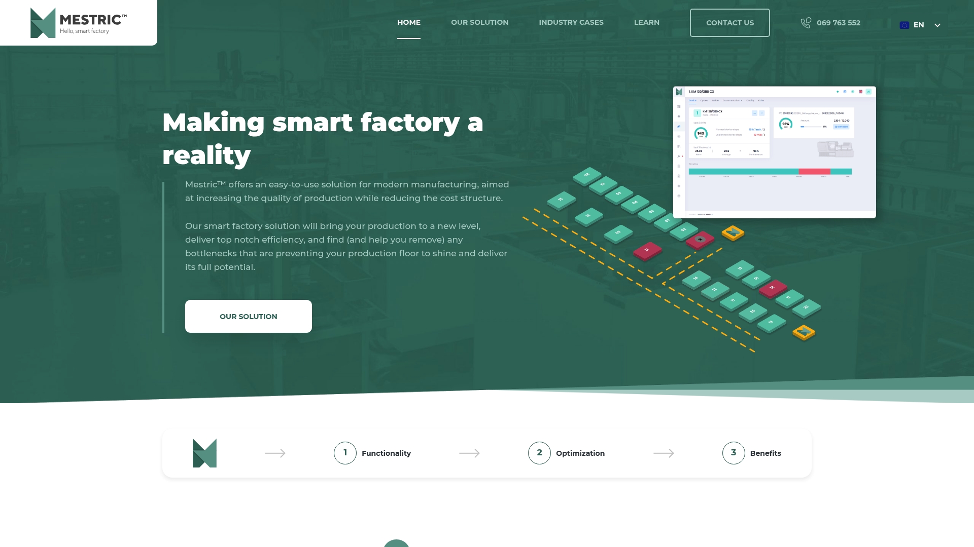
Where this guide recommends SLO-driven alerting, Mestric applies the same logic to production targets: define your throughput or quality SLO, connect your machines, and receive alerts when performance is burning through your acceptable deviation budget. The AI-powered optimisation layer identifies bottlenecks and suggests process adjustments, reducing the manual analysis burden on your operations team. If you are evaluating manufacturing software options for your plant, Mestric offers a personalised onsite demonstration so you can see connected machinery telemetry in a real production context. Request your demo at mestric.com.

Useful sources for further reading

The sources below informed this guide and are worth bookmarking for deeper technical detail.

• Microsoft Azure Well-Architected Framework: monitoring — the authoritative reference for hot/warm/cold telemetry architecture, UTC standardisation, and telemetry categorisation. Directly applicable to any cloud or hybrid UK deployment.
• Microsoft Azure Well-Architected Framework: reliability monitoring — explains why SLOs should drive alerting strategy rather than component-level thresholds. Essential reading for anyone designing an SLO-based monitoring programme.
• Real-Time Performance Monitoring at Scale (Alex Mayhew) — a practitioner post covering percentile-based latency, histogram aggregation, burn-rate alerting, and RUM/synthetic combinations. Concrete and technically detailed.
• Cloud Monitoring Best Practices (New Relic) — covers unified observability patterns, service maps, and the alert-to-trace-to-log workflow. Useful for teams evaluating integrated platforms.
• Monitoring best practices for developers (middleware.io) — practical guidance on log verbosity by environment and recovery testing cadence. Good reference for development teams new to production monitoring.
• Linux performance monitoring guide (clinux.tech) — covers server-level diagnostics using top, htop, vmstat, iostat, and sar alongside long-term collectors. Useful for on-call engineers diagnosing infrastructure-level bottlenecks.
• What is real-time performance monitoring? (Hyperbots) — a concise practitioner-facing definition useful as a quick reference.
• Troubleshoot issues using Performance Monitor (Microsoft Learn) — Windows-specific guidance for CPU, memory, and disk counter collection using Performance Monitor (perfmon). Relevant for teams running Windows Server workloads alongside cloud-native services.
• How to monitor performance: steps and best practices (Slack) — a broader treatment of performance monitoring that covers goal-setting, baselines, tooling selection, and communication. Useful for operations managers aligning technical monitoring with business objectives.
• Mestric: real-time performance tracking for manufacturing — maps the guide’s technical recommendations to a practical MES implementation, covering KPI tracking, quality monitoring, and machine integration for UK manufacturing operations.
• SaraWest contract manufacturing — relevant for organisations considering supplier-side monitoring integration as part of a broader supply chain visibility programme.

Recommended

• Seven proven benefits of real-time monitoring in manufacturing
• Real-time performance tracking for manufacturing efficiency
• Real-Time Production Monitoring: Transforming Manufacturing
• How to Improve Manufacturing Efficiency with MES Tools