


Production capacity is the maximum output your line, cell, or plant can deliver in a set period. Skip the theoretical maximum and calculate effective capacity instead: usable machine-hours divided by cycle time, then adjusted by OEE. That figure, not the nameplate number, is what belongs in your scheduling and sales conversations.
TL;DR:
- Effective capacity usually ranges from 60% to 80% of theoretical capacity after accounting for typical losses and downtime.
- OEE adjustments typically reduce theoretical capacity by 25 to 40%, providing more realistic planning figures.
- Capacity should be calculated at the bottleneck resource because it determines the entire line’s throughput regardless of other resources.
- Manual capacity calculations require monitoring over multiple weeks to avoid inaccurate data caused by short-term variations.
- Using automated tools like Mestric™ MES enables real-time capacity tracking and constraint identification, improving planning accuracy.
Not all “capacity” numbers mean the same thing, and mixing them up is the fastest way to promise a customer something your line cannot deliver. Each type answers a different question:
Overall Equipment Effectiveness (OEE) ties these together through three components: availability (uptime versus planned time), performance (actual speed versus ideal speed), and quality (good units versus total units produced). Multiply the three and you get OEE as a single percentage. A related metric, TEEP (Total Effective Equipment Performance), measures OEE against all calendar hours rather than just scheduled hours, which is useful if you’re weighing whether to add shifts.
As a guideline, realistic capacity typically lands at 60 to 80% of theoretical once you strip out the common losses every plant faces. A utilisation figure consistently above 85% usually signals you’re close to the constraint and should be watching for missed deliveries; below 60% often points to demand issues rather than capacity issues.

Three methods cover most planning situations, ranging from a five-minute manual check to a full finite-scheduling model. Pick based on how much data maturity and precision the decision actually needs.
Statistic: Every one percentage point improvement in OEE produces roughly a one percentage point increase in realistic capacity, which is why OEE work is often the cheapest lever available before anyone talks about buying new equipment.
Whichever method you use, always calculate at the level of the constraint resource, the single machine or work centre with the least spare time relative to demand. Capacity anywhere else in the line is largely irrelevant if the bottleneck can’t keep pace; our guide on identifying production bottlenecks walks through how to find it reliably.
Here’s a compact example using a single work centre running two machines across two shifts.
| Input | Value |
|---|---|
| Machines | 2 |
| Shifts per day | 2 |
| Net minutes per shift | 440 (after breaks) |
| Cycle time per unit | 1.5 minutes |
| Setup time per batch | 2 batches per shift |
| Planned downtime | 5% of shift time |
| OEE | 0.72 |
| Yield | 0.97 |
Working through it:
If actual demand booked against this work centre is 600 units a day, utilisation sits at roughly 83% (600 ÷ 723), comfortably inside a healthy operating band without leaving the line dangerously exposed to a bad shift. For a deeper look at converting cycle time into scheduling units, the takt time calculation guide is worth bookmarking alongside this example.
A capacity number is only as good as the inputs behind it, and the two most common errors are mixing rated speed with observed speed, and sampling too short a window to smooth out normal variation.
Pro Tip: Never trust a single “good day” sample. Pull your cycle time and downtime figures from at least three separate weeks, including one that includes a changeover-heavy day, before you commit a capacity number to a customer promise.
A spreadsheet works for a single line. Once you’re tracking several work centres or product families, an MES that automates data capture removes the guesswork entirely, and our capacity planning checklist covers exactly what to log before you trust the output.
Capital spending is rarely the first answer, and often the wrong one. Try these levers in order:
The formula is the easy part. The harder part is getting a capacity figure that survives contact with an S&OP meeting, where sales wants a bigger number and operations wants a safer one. Numbers built from demonstrated output tend to win arguments that theoretical numbers lose, because nobody can dispute what the line has already produced… Trust the historical floor before you trust the spreadsheet ceiling.
— Andraž
Every method above still depends on someone manually timing cycles, logging downtime codes, and reconciling spreadsheets after the shift ends. Mestric replaces that manual layer entirely by connecting directly to your equipment, capturing cycle time, downtime, and quality data automatically as production runs.
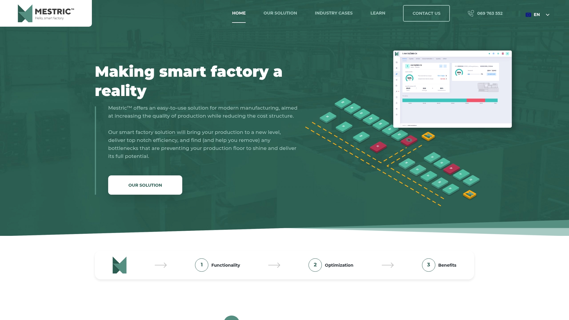
Instead of running an OEE calculation once a quarter from patchy logs, you get a live OEE dashboard that flags the constraint resource in real time and alerts you when a bottleneck is eating into effective capacity. That shortens the distance between “what our capacity should be” and “what our capacity actually is” from weeks of data reconciliation to a glance at the shop floor screen. If you want to see how this looks against your own production data, book a demonstration through the Mestric™ MES platform page and bring your current cycle-time assumptions along to test.
Divide usable machine-hours (machines multiplied by working hours) by cycle time to get theoretical units, then multiply by OEE to get a realistic figure. This machine-hour method is the fastest starting point before moving to RCCP or finite scheduling.
Most plants aim to run somewhere between 60% and 85% of effective capacity, since realistic capacity typically sits at 60 to 80% of theoretical once normal losses are accounted for. Consistently exceeding this range signals you’re near your constraint and at risk of missed deliveries.
OEE converts a theoretical capacity figure into a realistic one by multiplying available time divided by cycle time against the OEE percentage. It commonly reduces theoretical capacity by 25 to 40%, which is why effective capacity, not theoretical capacity, belongs in your scheduling decisions.
Use RCCP at the sales and operations planning horizon to quickly test whether a demand plan is feasible using routings and representative times. Switch to finite scheduling (APS/CRP) when you need a detailed, defensible shop-floor schedule that accounts for actual calendars and setup sequences.
Yes. Mestric™ MES connects to your equipment to capture cycle time, downtime, and quality data automatically, generating live OEE dashboards that flag your constraint resource without manual timing or spreadsheet reconciliation. Current pricing and demonstration details are available through the Mestric™ MES page.


 069 763 552