


Line balancing (in Slovenian, uravnoteženje proizvodne linije) means distributing the work on a line across workstations so that each station needs about the same time per cycle. You start from takt time, work out the minimum number of stations, assign tasks without breaking their sequence, and then check line efficiency and idle time. This guide takes you through each step with worked numbers, and shows how live production data keeps the balance from drifting after the project ends.
According to ETH Zurich course material, line balancing assigns tasks to workstations to minimise their number and the total idle time for a given output level. It matters most in repetitive line production, where specialised equipment works in a fixed sequence. The same source describes it as a tool for reducing unevenness (the lean term is mura) by giving each production step a similar amount of work.
In formal terms, the assembly line balancing problem is a set of tasks with fixed times that must be assigned to sequential stations. The order of tasks follows precedence relationships, and the key constraint is the cycle time available at each station, as the 2023 MDPI study by Breznik, Buchmeister and Vujica Herzog puts it. That study comes from Slovenian authors working on a real assembly line.
There are two practical reasons to balance, according to the DAAAM 2024 scientific book: efficient use of labour, and fairness, since one station working much harder than its neighbours causes problems of its own.
Typical signs that a line needs balancing:
If you recognise these, the first job is to find the slowest station. Our guide to identifying production bottlenecks covers that step in detail.
Takt time is the pace the customer sets. The Lean Enterprise Institute defines it as available production time divided by customer demand. Its example: 480 minutes per day and demand for 240 widgets per day gives two minutes per widget.
The detail that decides whether your figure is right is what counts as available time. Use time when the line is planned to run, and leave out breaks, meetings and time between shifts. A worked example from Rework shows it clearly: an 8-hour shift minus 60 minutes of breaks leaves 420 minutes, or 25,200 seconds. With demand of 180 units per shift, takt time is 25,200 ÷ 180 = 140 seconds per unit.
A few rules of thumb:
For more formulas and examples, see our page on takt time calculation.
Balancing is only as good as the times you feed into it. You need three inputs, in line with the NTNU course slides: the task times, a list of activities with a precedence diagram, and the required throughput.
Task times. Use a stopwatch study on several cycles, or a predetermined time standard. The Slovenian study mentioned above used the MTM (Methods-Time Measurement) standard, which assumes that basic movements in the correct sequence are faster and cause fewer errors. It recommended MTM-UAS for the observed assembly line.
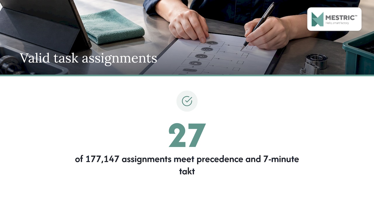
Precedence. List which task must finish before another can start. This is what makes balancing harder than simply sharing out work. In an example from KEVOS, 11 tasks across 3 stations allow 177,147 possible assignments, yet only 27 respect both the precedence rules and the 7.00-minute takt.
Variation. Single measurements hide variation between operators, shifts and product variants. Averages over many cycles are far more reliable. Collecting them by hand is slow, which is why many plants move cycle time capture to the machines themselves. Read more in our guide to cycle time measurement with an MES.
The theoretical minimum is total work content divided by takt time, rounded up, as Jodoo’s line balancing guide explains. Its example: 12 minutes of work content and a 2.5-minute takt gives 4.8, so you need at least 5 stations.
Treat this as a lower bound. Precedence rules and indivisible tasks usually mean the real answer is equal to it or slightly higher. The DAAAM book notes that tasks are assigned by eliminating those that do not fit the cycle time and those whose predecessors are not yet placed.
You do not need specialist software to start. Three heuristics cover most cases, all described in the sources above:
| Methode | How it works | Best used when |
|---|---|---|
| Largest Candidate Rule | Order tasks from longest to shortest. Open a station, add the longest task that is allowed by precedence and still fits, then open the next station when nothing fits. | You want a quick first solution by hand |
| Ranked Positional Weight | Rank each task by its own time plus the time of every task that follows it. Fill stations with the highest-ranked available task. | Precedence chains are long and the first rule leaves gaps |
| Kilbridge and Wester | Group tasks into precedence columns and assign by column. | The precedence diagram is clear and fairly linear |
A practical routine:
A feasible balance, as Scholl and Becker’s review states, is one where no station time exceeds the cycle time. Any station below it has idle time equal to the difference in each cycle.
Three numbers tell you whether the balance is good. Using the worked example from Jodoo (12 minutes of work, 5 stations, 2.5-minute takt):
The same source points out a trap: station 3 in that example takes 2.8 minutes, above the 2.5-minute takt. A high efficiency percentage does not make an infeasible station acceptable, so always check the longest station against takt first. The slowest station is the bottleneck and sets the real pace of the whole line.
A second example shows what a weaker result looks like. In an office chair assembly case from Lean 6 Sigma Hub, 23.7 minutes of total task time, 6 workstations and a 5-minute cycle give 79% balancing efficiency, which means 21% idle capacity.
Plants often use a Yamazumi chart, a stacked bar chart of the task times at each station against the takt line, to see this at a glance. Station bars above the line need work taken off. Bars far below it have spare capacity to receive work.
The figures below come from published studies. They show what is achievable in different settings, not what any particular plant will gain.
| Case | Methode | Result |
|---|---|---|
| Slovenian assembly line (MDPI, 2023) | MTM time standard and simulation | Difference between the bottleneck and the least occupied station cut from 38.37% to 8.52% |
| Wiring industry (ASTRJ, 2023) | DMAIC with Yamazumi chart | Line efficiency up from 78% to 95%, with a saving in manpower |
| Shoe finishing line (IJINS, 2024) | Largest Candidate Rule and Region Approach | Efficiency from 49.0% to 81.73%, stations from 15 to 9 |
| Automotive supplier in Slovakia (TEM Journal, 2024) | Yamazumi graph | Cycle time from 22.7 to 17.7 seconds, fewer operators needed |
The wiring study makes one point worth copying: build the Yamazumi diagram both before and after the changes, and judge the improvement by comparing the two efficiency values. Without a documented starting point you cannot show what the project delivered.
A line balanced on paper starts to drift on day one. A new variant changes task times. A machine slows down. An experienced operator leaves. Micro-stoppages move the bottleneck from one station to another. If you only re-measure once a year, you are balancing last year’s line.
That is why ongoing balancing needs three data streams:
Slovenian industry already shows how far data-driven layout work can go. At UNIOR in Zreče, a digital twin was used to optimise production layout and internal logistics, reportedly increasing the number of operations performed by more than 320% and reducing material transport distances by 43%. Few plants start with a digital twin, but the principle is the same: decisions about layout rest on measured data.
For related planning work, see our guides on production capacity planning und Schritt-für-Schritt-Produktionsoptimierung.
Most balancing projects we see are treated as a one-off exercise: a time study, a spreadsheet, a new station layout. The result is good for a few weeks. Then the product mix changes and nobody knows which station is now the slowest.
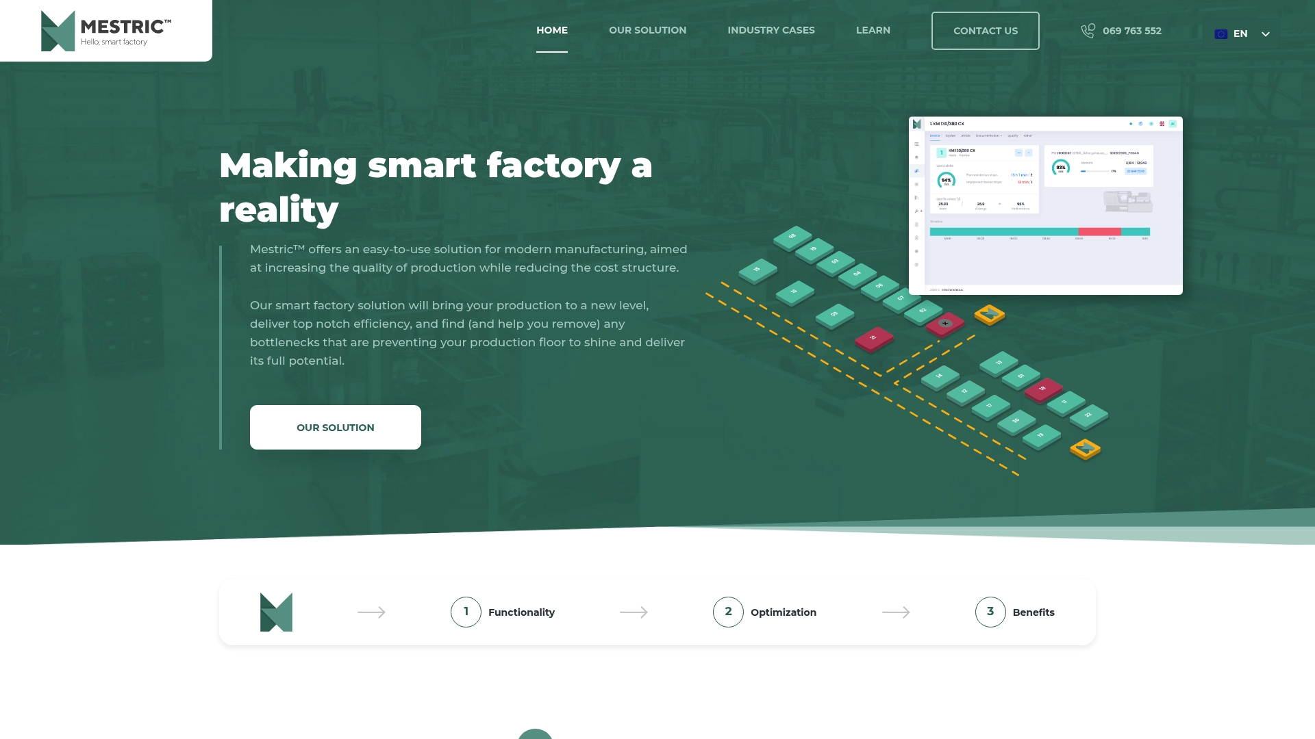
We built Mestric™ MES around a different idea. The system connects directly with your equipment, collects data automatically and shows KPIs such as performance, downtime and quality parameters in real time. Production managers see where the bottleneck is today, not where it was in the last study.
Our AI-powered optimisation tools are designed to support the decisions that follow: where to move work, which process norms to adjust, and which stoppages to attack first. Less manual data entry also means fewer manual errors in the very times your balance depends on.
Our advice: do the paper balance once, properly, with takt time and a Yamazumi chart. Then let live data tell you when it needs another look.
Andraž
If you want to see what station-level data looks like in practice, Mestric™ MES can be shown working with connected machinery. Our demonstration presents live KPI dashboards, downtime analysis and cost analytics in a real production setting, so you can judge how it would fit your line.
Read about the platform on our Mestric™ MES page, or see how real-time performance tracking supports daily decisions on the shop floor.
According to AMD Machines, 85–95% is generally considered good in practice, and below 80% signals significant rebalancing opportunities. Treat the range as a guide, since the right target depends on your process, variability and product mix.
Takt time is the pace set by customer demand: available time divided by demand. Cycle time is how long a station actually needs to complete its work. The line is on pace when the longest station cycle time does not exceed takt.
Divide total work content by takt time and round up. With 12 minutes of work and a 2.5-minute takt, you need at least 5 stations. The real number can be higher if precedence rules or indivisible tasks prevent a perfect fit.
Yes. A spreadsheet, a precedence diagram and a heuristic such as the Largest Candidate Rule are enough for a first balance. Software and live machine data become useful when you run many variants or need to keep the balance current over time.


 069 763 552